Eigenmodes of Helmholtz

Shared by Antoine Rideau

On this page you will find how to show using Castor the eigenmodes of the wave equation on a rectangle with fixed edges.

We start from the following D’Alembert equation on \(\Omega = \left [ 0, x_{0} \right ] \times \left [ 0, y_{0} \right ]\) with Dirichlet boundary condition on \(\Gamma = \partial \Omega\)

\[\begin{split}\left\{\begin{matrix} - \displaystyle \frac{1}{c} \frac{\partial^2 u }{\partial t^2}(\mathbf{x}) + \Delta u (\mathbf{x}) = 0 & , & \mathbf{x} \in \Omega \setminus \Gamma \\ u(\mathbf{x} , \cdot ) = 0 & , & \mathbf{x} \in \Gamma \end{matrix}\right. ,\end{split}\]

considering

\[u (\mathbf{x},t) = V(\mathbf{x})e^{i \omega t} ,\]

gives the Helmholtz equation

\[\begin{split} \left\{\begin{matrix} k^{2}V(\mathbf{x}) + \Delta V(\mathbf{x}) = 0 & , & \mathbf{x} \in \Omega \setminus \Gamma \\ V(\mathbf{x}) = 0 & , & \mathbf{x} \in \Gamma \end{matrix}\right. ,\end{split}\]

with \(k = \displaystyle \frac{\omega}{c}\) .

The space domain L is discretized with dx steps which results in the meshgrid described by X and Y

\[\begin{split}\begin{matrix} x_{i} = i \delta x & \text{ for } i = \left [ \! \left [ 0, n_{x}-1 \right ] \! \right ]\\ y_{j} = j \delta x & \text{ for } j = \left [ \! \left [ 0, n_{y}-1 \right ] \! \right ] \end{matrix}\end{split}\]

// Parameters
matrix<> L = {1, 2}; // Dimensions
double dx = 0.05;    // Space discretization

// Discretization
matrix<> X, Y;
std::tie(X, Y) = meshgrid(colon(0, dx, L(0)), colon(0, dx, L(1)));

See meshgrid.

Laplacian

The Helmholtz equation can now be written in vector form

\[- K V(\mathbf{x}) = k^{2} V(\mathbf{x}) ,\]

where K stands for the matrix of the Laplacian operator.

The Laplacian operator can be approximated as

\[\begin{split}\begin{matrix} \Delta_{\textbf{x}}u(x,y) & = & \displaystyle \frac{\partial^2 u}{\partial x^2}(x,y) + \frac{\partial^2 u}{\partial y^2}(x,y) \\ \Delta_{\textbf{x}}u_{i,j} & \approx & \displaystyle \frac{u_{i+1,j}+u_{i,j+1}-4u_{i,j}+u_{i-1,j}+u_{i,j-1}}{\delta_{\textbf{x}}^2} & . \end{matrix}\end{split}\]

This expression leads to this form for K

\[\begin{split}K = \frac{1}{\delta_{\textbf{x}}^2} \begin{pmatrix} -4 & 1 & 0 & \cdots & 0 & 1 & 0 & \cdots & 0\\ 1 & -4 & 1 & 0 & \cdots & 0 & 1 & \ddots & \vdots \\ 0 & 1 & \ddots & \ddots & \ddots & & \ddots & \ddots & 0\\ \vdots& \ddots & \ddots & -4 & 1 & 0 & & \ddots & 1\\ 0 & & 0 & 1 & -4 & 1 & 0 & & 0\\ 1& \ddots & & 0 & 1 & -4 & \ddots & \ddots & \vdots \\ 0 & \ddots & \ddots & & \ddots & \ddots & \ddots & 1 & 0 \\ \vdots& \ddots & 1 & 0 & \cdots & 0 & 1 & -4 & 1 \\ 0 & \cdots & 0 & 1 & 0 & \cdots & 0 & 1 & -4 \end{pmatrix} .\end{split}\]

// Laplacian
long nx = size(X, 2), ny = size(X, 1);
matrix<> e = ones(nx * ny, 5);
e(row(e), 2) = -4;
matrix<> K = full(spdiags(1. / (dx * dx) * e, {-nx, -1, 0, 1, nx}, nx * ny, nx * ny));

See label-spdiags

Here, K is built as a sparse matrix using spdiags because it is easier to do so but I convert it into a dense matrix because Castor don’t have a sparse solver yet.

In order to take into account the homogeneous Dirichlet condition on the boundary, penalization is used on the index where the boundaries are : index i such as X(i)==0, X(i)==L(0), Y(i)==0 and Y(i)==L(1) .

// Penalization on boundary (Homogeneous Dirichlet condition)
matrix<std::size_t> Ibnd;
Ibnd = find((X == 0) || (X == L(0)) || (Y == 0) || (Y == L(1)));
K(sub2ind(size(K), Ibnd, Ibnd)) = 1e6;

See find, sub2ind.

Analytical solution

An eigenmodes is caracterize by 2 positive integers \(m\) and \(n\) . Thus the eigenvalues are

\[\lambda_{m,n} = c\pi \sqrt{\frac{m^2}{x_{0}}+\frac{n^2}{y_{0}}}\]

and the corresponding eigenmode are

\[u_{m,n} = \sin \bigg(\frac{m\pi x}{x_{0}}\bigg) \sin \bigg(\frac{n\pi y}{y_{0}}\bigg)\]

// Analytical
auto Dth = zeros(nx, ny);
for (int m = 0; m < nx; m++)
{
    for (int n = 0; n < ny; n++)
    {
        Dth(m, n) = M_PI * sqrt(pow((m + 1) / L(0), 2) + pow((n + 1) / L(1), 2));
    }
}

See zeros .

Eigenmodes

Once the Laplacian matrix have been built , eigenvalues are easily acquired in the 1 by nx*ny vector D and eigenvectors in the nx*ny by nx*ny matrix V using the eig function

\[- K V(\mathbf{x}) = D V(\mathbf{x})\]

// Numerical eigen values and vectors
matrix<std::complex<double>> D, V;
std::tie(D, V) = eig(-K, "right");

See eig .

The eigenvalues considerated are these with an imaginary part null and a real part minimal. To do so eigenvalues and eigenvectors are sorted by ascending eigenvalues.

// Sort
matrix<std::size_t> I;
I = argsort(abs(real(D)));
D = eval(D(I));
V = eval(V(row(V), I));
matrix<std::size_t> Ith;
Ith = argsort(Dth);
Dth = eval(Dth(Ith));

See argsort , row .

Then for each eigenmodes f , only the real part of the corresponding eigenvector is taken.

// Visu
std::vector<figure> fig(5);
for (int f = 0; f < fig.size(); f++)
{
    matrix<double> Z = reshape(real(eval(V(row(V), f))), size(X, 1), size(X, 2));
    mesh(fig[f], X, Y, Z);
}

See reshape , mesh .

Code

Here you have all the code at once :

#include "castor/matrix.hpp"
#include "castor/smatrix.hpp"
#include "castor/linalg.hpp"
#include "castor/graphics.hpp"

using namespace castor;

int main(int argc, char const *argv[])
{
    // Parameters
    matrix<> L = {1, 2}; // Dimensions
    double dx = 0.05;    // Space discretization

    // Discretization
    matrix<> X, Y;
    std::tie(X, Y) = meshgrid(colon(0, dx, L(0)), colon(0, dx, L(1)));

    // Visu mesh
    figure fig1;
    mesh(fig1, X, Y, zeros(size(X)));

    // Laplacian
    long nx = size(X, 2), ny = size(X, 1);
    matrix<> e = ones(nx * ny, 5);
    e(row(e), 2) = -4;
    matrix<> K = full(spdiags(1. / (dx * dx) * e, {-nx, -1, 0, 1, nx}, nx * ny, nx * ny));

    // Penalization on boundary (Homogeneous Dirichlet condition)
    matrix<std::size_t> Ibnd;
    Ibnd = find((X == 0) || (X == L(0)) || (Y == 0) || (Y == L(1)));
    K(sub2ind(size(K), Ibnd, Ibnd)) = 1e6;

    // Analytical
    auto Dth = zeros(nx, ny);
    for (int m = 0; m < nx; m++)
    {
        for (int n = 0; n < ny; n++)
        {
            Dth(m, n) = M_PI * sqrt(pow((m + 1) / L(0), 2) + pow((n + 1) / L(1), 2));
        }
    }

    // Numerical eigen values and vectors
    matrix<std::complex<double>> D, V;
    std::tie(D, V) = eig(-K, "right");

    // Sort
    matrix<std::size_t> I;
    I = argsort(abs(real(D)));
    D = eval(D(I));
    V = eval(V(row(V), I));
    matrix<std::size_t> Ith;
    Ith = argsort(Dth);
    Dth = eval(Dth(Ith));

    // Visu
    std::vector<figure> fig(5);
    for (int f = 0; f < fig.size(); f++)
    {
        matrix<double> Z = reshape(real(eval(V(row(V), f))), size(X, 1), size(X, 2));
        mesh(fig[f], X, Y, Z);
    }

    // Results
    std::cout << "-- Numerical eigenvalues --" << endl;
    disp(sqrt(real(eval(D(range(0, fig.size()))))), 1, fig.size());
    std::cout << "-- Analytical eigenvalues --" << endl;
    disp(eval(Dth(range(0, fig.size()))), 1, fig.size());
    std::cout << "-- Relative errors --" << endl;
    auto errRelative = abs((sqrt(real(eval(D(range(0, fig.size()))))) - eval(Dth(range(0, fig.size())))) / eval(Dth(range(0, fig.size())))) * 100;
    disp(errRelative, 1, fig.size());

    drawnow(fig1);

    return 0;
}

With this code you should get these outputs :

-- Numerical eigenvalues --
Matrix 1x5 of type 'd' (40 B):
    3.50946      4.43845      5.65288      6.45167      7.00046
-- Analytical eigenvalues --
Matrix 1x5 of type 'd' (40 B):
    3.51241      4.44288      5.66359      6.47656      7.02481
-- Relative errors --
Matrix 1x5 of type 'd' (40 B):
    0.08379      0.09980      0.18906      0.38427      0.34671

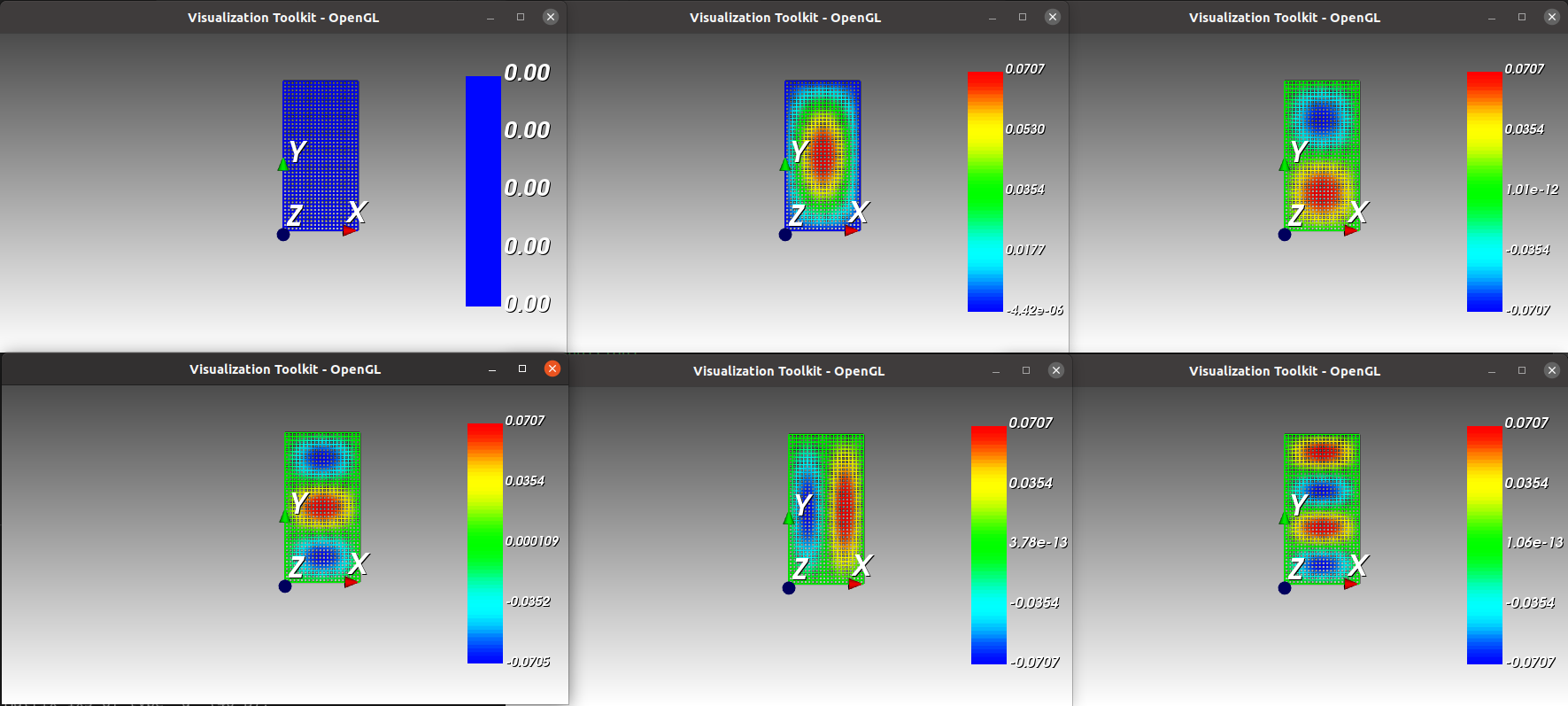
From up left corner to bottom right corner : the meshgrid and the five first eigenmodes.

References

http://ramanujan.math.trinity.edu/rdaileda/teach/s14/m3357/lectures/lecture_3_4_slides.pdf

http://www.cmap.polytechnique.fr/~jingrebeccali/frenchvietnammaster2_files/2017/LectureNotes/pde3d_mit.pdf