N-body problem
Shared by Antoine Rideau
|
|||
|---|---|---|---|
Sun and inner planet |
\(m_{0}\) = 1.00000597682 |
||
Jupiter |
\(m_{1}\) = 0.000954786104043 |
||
Saturn |
\(m_{2}\) = 0.000285583733151 |
||
Gravitational constant \(G = 2.95912208286 \times 10^{-4}\) |
|||
// Parameters
matrix<> m = {{1.00000597682}, {9.54786104043e-4}, {2.85583733151e-4}}; // Masses : Sun, Jupiter and Saturn
double G = 2.95912208286e-4;                                            //Gravitation's constant
The position of a object over time is given by \(q(t)\).
Bodies |
Initial position (AU) |
|---|---|
Sun |
0 |
0 |
|
0 |
|
Jupiter |
−3.5023653 |
−3.8169847 |
|
−1.5507963 |
|
Saturn |
9.0755314 |
−3.0458353 |
|
−1.6483708 |
where AU stands for astronomical unit and \(1 AU = 1.495 978 707 \times 10^{11}\) m.
matrix<> qini = {0, 0, 0,                               // Sun's initial position
                -3.5023653, -3.8169847, -1.5507963,     // Jupiter's initial position
                9.0755314, -3.0458353, -1.6483708};     // Saturn's initial position
Bodies |
Initial velocity (AU/day) |
|---|---|
Sun |
0 |
0 |
|
0 |
|
Jupiter |
0.00565429 |
0.00565429 |
|
−0.00190589 |
|
Saturn |
0.00168318 |
0.00483525 |
|
0.00192462 |
matrix<> vini = {0, 0, 0,                                                                   // Sun's initial velocity
0.00565429, -0.00412490, -0.00190589,                                                       // Jupiter's initial velocity
0.00168318, 0.00483525, 0.00192462};                                                        // Saturn's initial velocity
matrix<> pini = reshape(mtimes(transpose(m), ones(1, numel(m))), 1, numel(vini)) * vini;    // Initial momentums
See reshape , mtimes, transpose, ones, numel.
Time is discretized into nt steps
// Disretization
int nt = 1501;
double dt = (tend - tini) / (nt - 1);
auto T = linspace(tini, tend, nt);
See linspace.
Scheme
where
With such a separation, Hamilton equation are given by
where
which result to the symplectic Euler scheme :
// Scheme
auto Q = zeros(nt, numel(qini));
Q(0, col(Q)) = qini;
auto P = zeros(nt, numel(pini));
P(0, col(P)) = pini;
// Symplectic Euler
for (int it = 0; it < nt - 1; it++)
{
    matrix<> q_n = eval(Q(it, col(Q)));
    matrix<> p_n = eval(P(it, col(P)));
    Q(it + 1, col(Q)) = q_n + dt * H_p(G, m, p_n);
    P(it + 1, col(P)) = p_n - dt * H_q(G, m, eval(Q(it + 1, col(Q))));
}
In the code, \(\displaystyle \frac{\mathrm{d} K}{\mathrm{d} p}(p)\) is represented by the function H_p
matrix<> H_p(double G, matrix<> m, matrix<> p)
{
    auto Hp = zeros(1, numel(p));
    m = reshape(mtimes(transpose(m), ones(1, numel(m))), 1, numel(p));
    Hp = p / m;
    return Hp;
}
See zeros, reshape , mtimes, transpose, ones, numel.
and \(\displaystyle \frac{\mathrm{d} V}{\mathrm{d} q}(q)\) by the function H_q
matrix<> H_q(double G, matrix<> m, matrix<> q)
{

    auto q0 = eval(q(range(0, 3)));
    auto q1 = eval(q(range(3, 6)));
    auto q2 = eval(q(range(6, 9)));
    auto Hq = zeros(1, 9);
    Hq(range(0, 3)) = (G * m(0) * m(1) * ((q0 - q1) / pow(norm(q0 - q1), 3)) + G * m(0) * m(2) * ((q0 - q2) / pow(norm(q0 - q2), 3)));
    Hq(range(3, 6)) = (G * m(1) * m(0) * ((q1 - q0) / pow(norm(q1 - q0), 3)) + G * m(1) * m(2) * ((q1 - q2) / pow(norm(q1 - q2), 3)));
    Hq(range(6, 9)) = (G * m(2) * m(0) * ((q2 - q0) / pow(norm(q2 - q0), 3)) + G * m(2) * m(1) * ((q2 - q1) / pow(norm(q2 - q1), 3)));
    return Hq;
}
Visualisation
Simple figure with Castor
plot or plot3, here plot3 is used to show the motion in 3 dimensions.transpose is needed because of matrix Q ‘s dimensions.// Visu
figure fig;
plot3(fig, transpose(eval(Q(row(Q), 3)) - eval(Q(row(Q), 0))), transpose(eval(Q(row(Q), 4)) - eval(Q(row(Q), 1))), transpose(eval(Q(row(Q), 5)) - eval(Q(row(Q), 2))), {"c"});
plot3(fig, transpose(eval(Q(row(Q), 6)) - eval(Q(row(Q), 0))), transpose(eval(Q(row(Q), 7)) - eval(Q(row(Q), 1))), transpose(eval(Q(row(Q), 8)) - eval(Q(row(Q), 2))), {"b"});
plot3(fig, zeros(1, nt), zeros(1, nt), zeros(1, nt), {"y"});
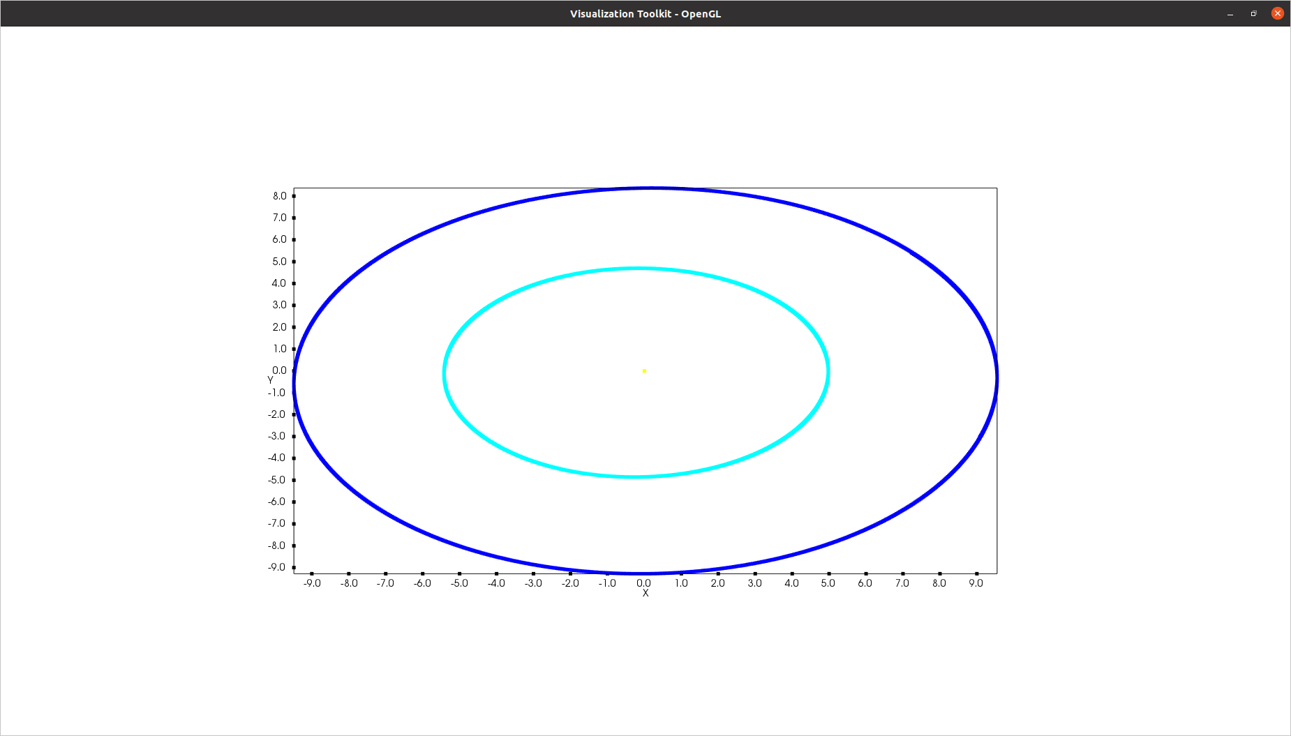
Orbits of Jupiter (cyan) and Saturn (blue) around the Sun (yellow) in the center.
Video output with VTK
// Initialize source and movie
vtkNew<vtkWindowToImageFilter> source;
vtkNew<vtkOggTheoraWriter> movie;
movie->SetInputConnection(source->GetOutputPort());
movie->SetFileName("nbody.avi");
movie->SetQuality(2); // in [0,2]
movie->SetRate(25);   // frame per seconds
int Nplot = 150;      // < 200
Afterwards, the writer is initiated before the loop over time.
movie->Start();
for (int it = 0; it < nt - 1; it++){...}
Then each wanted frame is plotted and added to the final movie.
// Visu
if (it % (nt / Nplot) == 0)
{
    figure fig;
    matrix<> limits = {-10, 10};
    plot(fig, {Q(it, 3) - Q(it, 0)}, {Q(it, 4) - Q(it, 1)}, {"c"});
    plot(fig, {Q(it, 6) - Q(it, 0)}, {Q(it, 7) - Q(it, 1)}, {"b"});
    plot(fig, zeros(1), zeros(1), {"y"});
    xlim(fig, limits);
    ylim(fig, limits);
    source->SetInput(fig.GetView()->GetRenderWindow());
    source->SetInputBufferTypeToRGB();
    source->ReadFrontBufferOff();
    movie->Write();
}
See plot, label-xlim, label-ylim.
Finally, the writer is closed after the loop over time.
for (int it = 0; it < nt - 1; it++){...}
movie->End();
Video animation with Python
Q are stored in a .txt file using writetxt .// Output
writetxt("./", "dataJu.txt", cat(2, eval(Q(row(Q), 3)) - eval(Q(row(Q), 0)), eval(Q(row(Q), 4)) - eval(Q(row(Q), 1))));
writetxt("./", "dataSa.txt", cat(2, eval(Q(row(Q), 6)) - eval(Q(row(Q), 0)), eval(Q(row(Q), 7)) - eval(Q(row(Q), 1))));
Then the following Python code shows the beautiful animation.
import matplotlib.pyplot as plt
import matplotlib.animation as animation
import numpy as np
from collections import deque

# Data input
dataJu = np.loadtxt("./build/dataJu.txt")
dataSa = np.loadtxt("./build/dataSa.txt")

# Parameters extraction
nt = int(dataJu[0, 0])

# Data processing
dataJu = np.delete(dataJu, 0, 0)
dataSa = np.delete(dataSa, 0, 0)

# Visu initialization
fig = plt.figure(figsize=(5, 4))
ax = fig.add_subplot(autoscale_on=False, xlim=(-10, 10), ylim=(-10, 10))
ax.set_aspect('equal')

line, = ax.plot([], [], 'o', lw=2)
traceJu, = ax.plot([], [], ',-', lw=1)
traceSa, = ax.plot([], [], ',-', lw=1)
historyJu_x, historyJu_y = deque(maxlen=nt), deque(maxlen=nt)
historySa_x, historySa_y = deque(maxlen=nt), deque(maxlen=nt)


def animate(i):
    # Get planets' current positions
    thisx = [0, dataJu[i, 0], dataSa[i, 0]]
    thisy = [0, dataJu[i, 1], dataSa[i, 1]]

    # Clear the trace when the animation loops
    if i == 0:
        historyJu_x.clear()
        historyJu_y.clear()
        historySa_x.clear()
        historySa_y.clear()

    # Add the current position to the trace
    historyJu_x.appendleft(thisx[1])
    historyJu_y.appendleft(thisy[1])
    historySa_x.appendleft(thisx[2])
    historySa_y.appendleft(thisy[2])

    line.set_data(thisx, thisy)  # Update planets' positions
    # Update planets' traces
    traceJu.set_data(historyJu_x, historyJu_y)
    traceSa.set_data(historySa_x, historySa_y)
    return line, traceJu, traceSa


# Creating the Animation object
ani = animation.FuncAnimation(
    fig, animate, nt, interval=10, blit=True)
plt.show()
Code
Here is all the code at once, without the functions H_q and H_p written above :
#include "castor/matrix.hpp"
#include "castor/graphics.hpp"
#include "castor/linalg.hpp"

using namespace castor;

    int main(int argc, char const *argv[])
{
    // Parameters
    matrix<> m = {1.00000597682, 9.54786104043e-4, 2.85583733151e-4}; // Masses : Sun, Jupiter and Saturn
    double G = 2.95912208286e-4;                                      //Gravitation's constant

    matrix<> qini = {0, 0, 0,                                                                // Sun's initial position
                     -3.5023653, -3.8169847, -1.5507963,                                     // Jupiter's initial position
                     9.0755314, -3.0458353, -1.6483708};                                     // Saturn's initial position
    matrix<> vini = {0, 0, 0,                                                                // Sun's initial velocity
                     0.00565429, -0.00412490, -0.00190589,                                   // Jupiter's initial velocity
                     0.00168318, 0.00483525, 0.00192462};                                    // Saturn's initial velocity
    matrix<> pini = reshape(mtimes(transpose(m), ones(1, numel(m))), 1, numel(vini)) * vini; // Initial momentums

    double tini = 0.;
    double tend = 12500.;

    // Disretization
    int nt = 1501;
    double dt = (tend - tini) / (nt - 1);
    auto T = linspace(tini, tend, nt);

    // Initialize source and movie
    vtkNew<vtkWindowToImageFilter> source;
    vtkNew<vtkOggTheoraWriter> movie;
    movie->SetInputConnection(source->GetOutputPort());
    movie->SetFileName("nbody.avi");
    movie->SetQuality(2); // in [0,2]
    movie->SetRate(25);   // frame per seconds
    int Nplot = 150;      // < 200

    // Scheme
    auto Q = zeros(nt, numel(qini));
    Q(0, col(Q)) = qini;
    auto P = zeros(nt, numel(pini));
    P(0, col(P)) = pini;
    // Symplectic Euler
    tic();
    movie->Start();
    for (int it = 0; it < nt - 1; it++)
    {

        matrix<> q_n = eval(Q(it, col(Q)));
        matrix<> p_n = eval(P(it, col(P)));
        Q(it + 1, col(Q)) = q_n + dt * H_p(G, m, p_n);
        P(it + 1, col(P)) = p_n - dt * H_q(G, m, eval(Q(it + 1, col(Q))));

        // Visu
        if (it % (nt / Nplot) == 0)
        {
            figure fig;
            matrix<> L({-10, 10, -10, 10}); // Axis dimensions
            plot(fig, Q(it, 3) - Q(it, 0) * ones(1), Q(it, 4) - Q(it, 1) * ones(1), L, {"c"});
            plot(fig, Q(it, 6) - Q(it, 0) * ones(1), Q(it, 7) - Q(it, 1) * ones(1), L, {"b"});
            plot(fig, zeros(1), zeros(1), {"y"});
            source->SetInput(fig.GetView()->GetRenderWindow());
            source->SetInputBufferTypeToRGB();
            source->ReadFrontBufferOff();
            movie->Write();
        }
    }
    movie->End();
    toc();

    // Output for Python post-processing and visualisation
    // writetxt("./", "dataJu.txt", cat(2, eval(Q(row(Q), 3)) - eval(Q(row(Q), 0)), eval(Q(row(Q), 4)) - eval(Q(row(Q), 1))));
    // writetxt("./", "dataSa.txt", cat(2, eval(Q(row(Q), 6)) - eval(Q(row(Q), 0)), eval(Q(row(Q), 7)) - eval(Q(row(Q), 1))));

    // Visu in native Castor
    // figure fig;
    // plot3(fig, transpose(eval(Q(row(Q), 3)) - eval(Q(row(Q), 0))), transpose(eval(Q(row(Q), 4)) - eval(Q(row(Q), 1))), transpose(eval(Q(row(Q), 5)) - eval(Q(row(Q), 2))), {"c"});
    // plot3(fig, transpose(eval(Q(row(Q), 6)) - eval(Q(row(Q), 0))), transpose(eval(Q(row(Q), 7)) - eval(Q(row(Q), 1))), transpose(eval(Q(row(Q), 8)) - eval(Q(row(Q), 2))), {"b"});
    // plot3(fig, zeros(1, nt), zeros(1, nt), zeros(1, nt), {"y"});

    // drawnow(fig);

    return 0;
}