Plotting and much more
We describe here some aspects of the graphics library available within the castor project. It is based on the well-known VTK library which must be installed by the user. Depending on the operating system, binary files may be directly available. However, one should pay attention to the fact that it is only compatible with version 9.x.
After installing VTK (see Installation), the user only needs to include the castor/graphics.hpp header file.
The path is very close to the one chosen by Matlab or Matplotlib (for the Python language). First, the user creates a figure which is a container which will hold the plots. Then,he adds one or multiple plots to the figure. Finally, he asks the system to display the figures (one window per figure will be created) with the drawnow(...) function. Each call to drawnow displays all the figure objects which have been defined since the last call.
Warning
Each call to drawnow is blocking, meaning that it will suspend the execution of the program until all the opened figure are closed.
This behavior cannot be modified as it is due to VTK.
On Windows and linux, when the opened figure are closed, the program stops. A workaround consists in to call the drawnow` function at the end
of the program.
The graphics library features 2D/3D customizable plotting and basic triangular/tetrahedral mesh generation. We detail the use of some of these features below. The demo files may be found in the demo/demo_graphics/ subfolder.
It is possible to interact with the figures in multiple ways:
“right-click and hold” : rotate the content in the direction of the mouse-pointer for 3D figures. For 2D plots, the user can use it to drag the plots in the direction of choice.
“middle-click and hold”: translate the content in the direction of the mouse-pointer.
“left-click and hold”: zoom-in if the pointer is in the upper window, otherwise zoom-out.
“key-pressed e or q”: close window. Warning: in some systems, it closes all windows.
“key-pressed r”: resets the view.
“key-pressed w”: switches to wireframe view when applicable.
“key-pressed s”: switches to surface view when applicable.
We advise the user to experiment with the different features mentioned above. The summary of all the available functions is available at Basic plot, Graphical input/output, Graphical tools, Mesh management and Mesh plot.
Basic 2D plotting
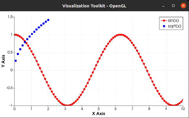
In this example, we will plot a sine and a square root function with different styles but on the same display. First, we initialize some data and we create a figure object. The full code is available at demo/demo_graphics/basic.cpp.
matrix<> X = linspace(0,10,100);
matrix<> Y = cos(X);
figure fig;
Then, we add our first plot as a red solid line with diamond markers with the correct legend.
plot(fig,X,Y,{"r-d"},{"sin(x)"});
Now we create a second set of data, reusing the already-defined variables. This is possible because the inputs are copied. This time, we plot it as a simple dotted blue line.
X = linspace(-2,2,30);
Y = sqrt(X);
plot(fig,X,Y,{"b"},{"sqrt(x)"});
// display
drawnow(fig);
The figure should look like this:
Remark: Currently, it is not possible to save the output to a graphic file.
Surface plot
Surface plotting consists in plotting a surface defined by the equation Z = f(X,Y). First we create the grid (X,Y). The full code is available at demo/demo_graphics/surface_plot.cpp.
matrix<> X,Y;
std::tie(X,Y) = meshgrid(linspace(-M_PI,M_PI,100));
Then, we create the surface which we want to plot, create a figure, adjust the color axis and display everything.
matrix<> Z = 2*sin(X)/X * sin(Y)/Y;
// create the figure
figure fig;
caxis(fig,{-1,1}); // scaled color in the range [-1,1]
mesh(fig,X,Y,Z);
// display
drawnow(fig);
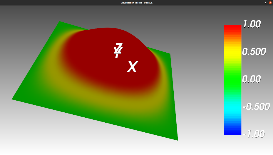
The result is a 3-dimensional plot which should look like this :
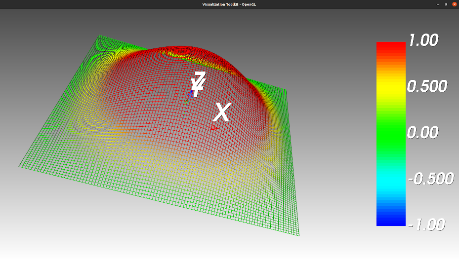
TIP: It is possible to switch to a full surface plot by pressing the s key and switch back to a wireframe display by pressing the w key.
Displaying nodal values
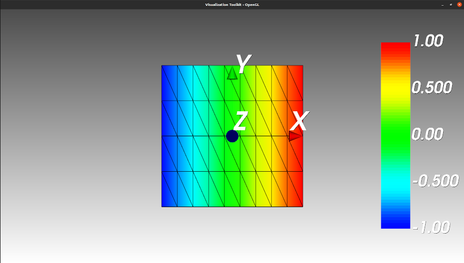
This feature is particularly useful if, for example, one needs to display the result of a finite element computation where the data is known at the vertices. In the following example, we create a planar mesh with triangular elements. Then we define a linearly increasing nodal data along the x-axis. The full code is available at demo/demo_graphics/nodal_values.cpp.
// geometric data
matrix<> X,Y;
std::tie(X,Y) = meshgrid(linspace(-1,1,10),linspace(-1,1,5));
X = vertcat(X,X);
Y = vertcat(Y,Y);
matrix<> Z = zeros(size(X));

// create mesh
matrix<> vtx;
matrix<std::size_t> elt;
std::tie(elt,vtx) = tridelaunay(X,Y,Z);

// display
figure fig;
trimesh(fig,elt,vtx,eval(vtx(row(vtx),0)));
drawnow(fig);
The result should look like this:
From mesh generation to file output
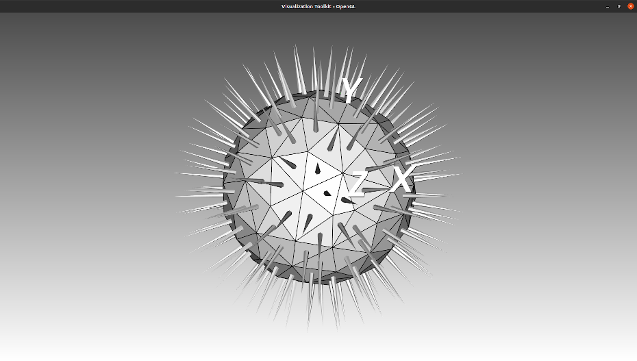
In this example, we create a spherical mesh and compute the normals to the triangles. We plot both on the same figure. Finally, we save the mesh to a .ply file. We also illustrate the use of the quiver function. The full code is available at demo/demo_graphics/advanced_mesh.cpp.
First, we create the mesh using the sphere2 function which creates a Fibonacci sphere.
std::size_t nvtx=100;
// 1. Create the mesh
matrix<> vtx;
matrix<std::size_t> elt;

matrix<> X,Y,Z;
std::tie(X,Y,Z) = sphere2(nvtx); // Fibonacci sphere
// Delaunay tetrahedrisation
std::tie(elt,vtx) = tetdelaunay(X,Y,Z);
// Boundary extraction
std::tie(elt,vtx) = tetboundary(elt,vtx);
Then, we compute the center ctr of the triangles and the normal vector nrm. We recall that the coordinates of ctr are simply the averaged sum of the coordinates of the vertices of the triangles. The coordinates of nrm may be determined by computing the cross-product between the tangent of, two consecutive edges. In this example we normalize the length to 0.25 to get an equilibrated display.
// 2. Compute the normal vectors and the centers of the triangles
std::size_t nelt = size(elt,1);
matrix<> nrm = zeros(nelt,3);
matrix<> ctr = zeros(nelt,3);
for(std::size_t ie=0; ie<nelt; ++ie)
{
    // center
    for(std::size_t i=0; i<3; ++i)
    {
        ctr(ie,i) = (vtx(elt(ie,0),i)+vtx(elt(ie,1),i)+vtx(elt(ie,2),i))/3.;
    }
    // normal vector to triangle {A,B,C}
    matrix<> AB=zeros(1,3), BC=zeros(1,3), nv = zeros(1,3);
    for(std::size_t i=0; i<3; ++i)
    {
        // tangent to first edge
        AB(i) = vtx(elt(ie,1),i) - vtx(elt(ie,0),i);
        tangent to second edge
        BC(i) = vtx(elt(ie,2),i) - vtx(elt(ie,1),i);
    }
    // for single vectors, this code is faster than
    // a call to 'cross' (for the cross-product) or 'norm'.
    nv(0) = AB(1)*BC(2) - AB(2)*BC(1);
    nv(1) = AB(2)*BC(0) - AB(0)*BC(2);
    nv(2) = AB(0)*BC(1) - AB(1)*BC(0);
    double l = std::sqrt(nv(0)*nv(0)+nv(1)*nv(1)+nv(2)*nv(2));
    // normalization
    for(std::size_t i=0; i<3; ++i)
    {
        nrm(ie,i) = nv(i)/(2*l); // arrows of length 0.5
    }
}
Now, we plot the result.
// 3. Plot everything
figure fig;
trimesh(fig,elt,vtx); // plot the mesh
quiver(fig,ctr,nrm);  // plot the normal vectors at the centers
drawnow(fig);
Finally, save the mesh into the current directory in the .ply format.
// 4. save to .ply
std::string path="./", name="testfile.ply";
triwrite(path,name,elt,vtx);
The result should look like an urchin, see below. Please note that the normal vectors may not appear when the window appears. In that case, simply clicking inside the window should do the trick.